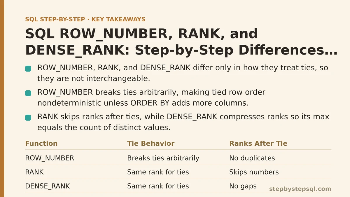
A common misconception is that ROW_NUMBER, RANK, and DENSE_RANK are basically interchangeable ranking functions, and that picking one over another is a matter of personal preference. They are not interchangeable. They produce different numbers on the same data, and choosing the wrong one silently changes which rows your downstream filter keeps.
The three functions share the same OVER (…) shape, share the same PARTITION BY and ORDER BY clauses, and share the same purpose of assigning a position to each row within a group. The only thing that separates them is how they treat ties. That single detail is what makes them behave so differently once you add a WHERE clause on top of the result.
The rest of this tutorial works through one concrete dataset from setup to a filtered result, so the differences show up in the output instead of staying abstract.
Setting Up a Small Sales Table
Start with a minimal sales table. Four regions, and within each region a handful of transactions with slightly different amounts. The point is to have at least one real tie inside a partition, because ties are where the three functions diverge.
CREATE TABLE sales (
    region       VARCHAR(20),
    salesperson  VARCHAR(20),
    amount       DECIMAL(10,2)
);

INSERT INTO sales (region, salesperson, amount) VALUES
    ('North', 'Alice',   500.00),
    ('North', 'Bob',     500.00),
    ('North', 'Carol',   300.00),
    ('North', 'Dan',     200.00),
    ('South', 'Erin',    800.00),
    ('South', 'Frank',   600.00),
    ('South', 'Grace',   600.00),
    ('South', 'Henry',   100.00);
Two things are deliberate here. Alice and Bob tie at 500 in the North region. Frank and Grace tie at 600 in the South region. Every region has a clear top and a clear bottom, so the shape of the ranked output will be easy to read.
If you run SELECT * FROM sales ORDER BY region, amount DESC; you get eight rows back. That is the row-level detail. The ranked columns come next.
Adding the Three Ranking Functions Side by Side
The step that makes these functions click is putting all three into the same query. Same partition, same order, three columns of output.
SELECT
    region,
    salesperson,
    amount,
    ROW_NUMBER() OVER (PARTITION BY region ORDER BY amount DESC) AS rn,
    RANK()       OVER (PARTITION BY region ORDER BY amount DESC) AS rnk,
    DENSE_RANK() OVER (PARTITION BY region ORDER BY amount DESC) AS dense_rnk
FROM sales
ORDER BY region, amount DESC;
When you run this, focus on the tied rows. In the North region, Alice and Bob both sit at 500. In the South region, Frank and Grace both sit at 600. Those are the only two places where the three columns disagree — everywhere else they agree row for row.
Roughly what you will see, trimmed to the North rows to keep it readable:
region | salesperson | amount | rn | rnk | dense_rnk
-------+-------------+--------+----+-----+----------
North  | Alice       | 500.00 |  1 |   1 |         1
North  | Bob         | 500.00 |  2 |   1 |         1
North  | Carol       | 300.00 |  3 |   3 |         2
North  | Dan         | 200.00 |  4 |   4 |         3
Walk through what the numbers are telling you.
ROW_NUMBER assigned Alice 1 and Bob 2. It broke the tie arbitrarily — whichever row the database happened to process first got the lower number. There is no rule that says Alice goes ahead of Bob; the ORDER BY only specifies amount DESC, and their amounts are equal, so the tiebreaker is undefined. This is the point most people miss. ROW_NUMBER never returns duplicates, but that guarantee comes with a hidden cost: for tied rows, the output is not deterministic across runs unless you add more columns to the ORDER BY.
RANK gave Alice and Bob both rank 1, then jumped Carol straight to rank 3. That gap at 2 is not a bug. It reflects the fact that two rows occupy the first position, so the next distinct value is pushing down to position 3 in the overall ordering.
DENSE_RANK also gave Alice and Bob rank 1, but then gave Carol rank 2. It compresses the sequence, so the highest number you will ever see inside a partition is the count of distinct values, not the count of rows.
The same pattern plays out in the South region: Erin takes the top spot at 800, Frank and Grace tie for second, Henry lands last.
How the Difference Shows Up in a Real Query
The reason this distinction matters is that people rarely select a ranked column and stop there. They filter on it. Change the filter, and the three functions give you three different row counts.
Suppose the question is: show me each region’s top performer. Filter for rn = 1 and you get one row per region.
SELECT region, salesperson, amount
FROM (
    SELECT
        region,
        salesperson,
        amount,
        ROW_NUMBER() OVER (PARTITION BY region ORDER BY amount DESC) AS rn
    FROM sales
) ranked
WHERE rn = 1;
Two rows come back — Alice (or Bob, depending on execution order) from the North, Erin from the South. One person per region, exactly as asked.
Now change that inner expression to RANK() and keep WHERE rn = 1. You get three rows back: Alice, Bob, and Erin. Because RANK assigned both tied leaders the value 1, the filter for 1 keeps both of them. If the business question was “show me the single top seller per region,” RANK just broke it. If the business question was “show me everyone tied for the top spot,” RANK is exactly right.
Change it to DENSE_RANK() with WHERE rn = 1. Same three rows as RANK in this dataset, because the filter is 1 either way. The two functions differ on subsequent positions, not on the top.
The lesson is direct: the filter value you write has to match the semantics of the function you chose. Filtering on value <= 3 against RANK gives you the top three finishers including ties; against ROW_NUMBER it gives you exactly three rows; against DENSE_RANK it gives you the top three distinct scores, which might be four or five rows if ties exist.
Deterministic Ties: When ROW_NUMBER Needs a Bouncer
If you need exactly one row per partition — a common reporting requirement, like “the most recent order per customer” — ROW_NUMBER is the right tool, but it needs help. Its tie-breaking behavior is unspecified, so on a dataset with duplicates it can return Alice today and Bob tomorrow.
The fix is to extend the ORDER BY with a unique column. In practice that means appending something like a primary key, an ID, or a timestamp that never collides within the partition.
SELECT
    region,
    salesperson,
    amount,
    ROW_NUMBER() OVER (
        PARTITION BY region
        ORDER BY amount DESC, salesperson ASC
    ) AS rn
FROM sales;
Adding salesperson ASC as a secondary sort key guarantees a stable result. Alice now wins the North region every time the query runs, because ‘Alice’ sorts before ‘Bob’ when amounts are equal.
Without that secondary key, the output is only guaranteed to be a correct answer, not the specific answer the business expects. That distinction gets people into trouble when a report needs to be reproducible — auditing it later and getting a different name in the top slot looks like a bug.
Where RANK and DENSE_RANK Divergence Is the Point
RANK and DENSE_RANK only split from each other when there are ties below the top of the partition. In the sample data, that split does not show up because every partition has its top tie back-to-back with no second tie. Add one more row to see it clearly.
INSERT INTO sales (region, salesperson, amount) VALUES
    ('North', 'Ivan', 300.00);
Now Carol and Ivan tie for third in the North region. Re-run the full three-column query, and the North ranking becomes:
salesperson | amount | rn | rnk | dense_rnk
------------+--------+----+-----+----------
Alice       | 500.00 |  1 |   1 |         1
Bob         | 500.00 |  2 |   1 |         1
Carol       | 300.00 |  3 |   3 |         2
Ivan        | 300.00 |  4 |   3 |         2
Dan         | 200.00 |  5 |   5 |         3
Three distinct scores — 500, 300, 200 — produce three DENSE_RANK values and five RANK values. The gap after the second tie (jumping from 3 to 5) is RANK’s way of saying “two positions were consumed.” DENSE_RANK ignores the gap and counts scores, not positions.
Concretely, this means a filter like dense_rnk <= 3 gives you every salesperson in the North region, because there are only three distinct amounts. The equivalent rnk <= 3 filter drops Dan, because he landed at position 5. Both of those are reasonable answers, but they answer different questions. “Top three distinct sales levels” and “top three finishing positions including ties” are not the same request.
Choosing Between the Three
The deciding question is not which function is more powerful — they all do roughly the same work. The deciding question is how you want ties represented in the output, because that is the only behavior that differs.
Reach for ROW_NUMBER when you need a unique integer per row and ties should not exist at that level of granularity — most-recent-record-per-group, first-transaction-per-customer, and similar deduplication tasks. Always pair it with a deterministic secondary sort key, or accept that the result may vary between executions.
Reach for RANK when tied rows should share a rank and you want the sequence to reflect how many rows occupied higher positions. Leaderboards, competition scoring, and any report where “two people tied for first, so nobody is second” is the correct interpretation fit here.
Reach for DENSE_RANK when tied rows should share a rank and you want the numbering to count distinct buckets rather than physical positions. Tiering and segmentation work — top tier, second tier, third tier — reads more naturally as DENSE_RANK, because the tier numbers stay compact even when ties exist inside a tier.
None of the three is a good fit if you want rankings computed across a sliding range rather than the whole partition. RANK, DENSE_RANK, and ROW_NUMBER all operate on the entire partition defined by PARTITION BY; if your question involves “top 3 within the trailing 90 days ending on this row’s date,” a window frame clause is needed, and that is a different tutorial.
A Note on NULL and Duplicate Ordering
Two details that catch people off guard. First, ORDER BY amount DESC places NULL amounts at the top in some databases (PostgreSQL, Oracle default) and at the bottom in others (SQL Server with ASC ordering, MySQL with DESC, though behavior varies). If your amount column can be NULL, add NULLS LAST (or the equivalent for your dialect) if you care about where those rows land. Otherwise your “top 1” filter may return a row with a NULL amount.
Second, PARTITION BY with no ORDER BY at all is valid syntax but rarely what you want. Without ORDER BY, ROW_NUMBER still returns unique numbers, but the assignment is arbitrary — the database has no mandate for which row gets which number. RANK and DENSE_RANK, without an ORDER BY, treat every row in the partition as a tie, so RANK returns 1 for all of them and DENSE_RANK returns 1 for all of them. The output is technically correct and almost certainly useless. Always include an ORDER BY unless you have a specific reason not to.
Putting the Implementation Path Together
The workflow that keeps these functions straight is a short one, and it is worth following every time you use them:
- Write the partitioned ranking query without a filter, and SELECT all three columns side by side. Run it against the actual data.
- Look at the tied rows. Decide whether the ties should share a rank (RANK or DENSE_RANK) or be broken arbitrarily-then-deterministically (ROW_NUMBER plus a secondary sort key).
- Decide whether the sequence should count physical positions (RANK) or distinct values (DENSE_RANK).
- Only then add the outer filter, and check how many rows come back against what you expect.
Skipping step one is what leads to the “I filtered for rn = 1 and got three rows” surprise. Writing all three columns first turns an invisible choice into a visible one.
What does your data look like around the tie points — are ties meaningful for the question, or are they just noise in the source? If you describe the ranking question and the shape of your data, the correct choice between the three functions usually becomes obvious.
Related guides: SQL Window Functions Explained Simply: The Concept That Unlocks Advanced Reporting, SQL RANK vs DENSE_RANK vs ROW_NUMBER: How to Choose the Right One, and Beginners Guide to SQL Window Functions: ROW_NUMBER and RANK Explained.